NumPy入门笔记,NumPy官网这篇 Tutorial 的整理和补充
Table of Contents
- 1 基础知识
- 2 形状操作
- 3 副本与视图
- 4 进阶内容
- 5 高级索引及索引技巧
- 6 线性代数
- 7 技巧和提示
- 8 index
- 9 以下为补充内容
- 10 函数理解
- 11 特定任务
- 12 问题与分析
- 12.1
numpy.sort与numpy.argsort - 12.2
outer - 12.3
numpy.where,numpy.nonzero和numpy.argwhere - 12.4
mgrid,ogrid,meshgrid,ndenumerate与indices - 12.5
allclose与array_equal - 12.6 ndarray 和 matrix
- 12.7 reshape后自动降维
- 12.8 (n, )和(n, 1)的广播原则
- 12.9
tile和repeat - 12.10 只有一个数字的ndarray
- 12.11 NumPy性能对比
- 12.12 NumPy交换数据和比较操作
- 12.13 NumPy中的reshape操作
- 12.14 索引(indexing)与高级索引(advanced indexing, fancy indexing)的区别及特殊情况分析
- 12.15 获取指定行列交叉点上的数据
- 12.16 ndarray的链式索引
- 12.17 ndarray内存排布的深入理解
- 12.1
import numpy as np
import matplotlib.pyplot as plt

from IPython.core.interactiveshell import InteractiveShell
InteractiveShell.ast_node_interactivity = "all"
基础知识
NumPy中主要的数据格式叫做ndarray,或者叫array,顾名思义即多维数组。
一个例子
ndarray的一些属性
- ndarray.ndim 维度
- ndarray.shape 形状,比如3维数组可能的形状(3,3,2)
- ndarray.size ndarray中的元素数
- ndarray.dtype ndarray中元素的数据类型
- ndarray.itemsize 每一个元素的字节数,等价于
ndarray.dtype.itemsize - ndarray.data 实际存储 ndarray 内容的内存
- ndarray.T ndarray的转置,一个视图(view, 类似于引用),下文统称视图.
- ndarray.flat 返回ndarray的一维化迭代器,对此迭代器赋值将导致整个数组元素被覆盖,而
ndarray.flatten()返回一个一维化的ndarray副本 - ndarray.real/imag 返回复数数组的实部/虚部数组
- ndarray.nbytes 数组占用的字节数
- ndarray.base 返回父 ndarray,如果该ndarray是其他 ndarray 的 view,则返回原始的 ndarray
- ndarray.flags ndarray的基本信息,是否对底层数据具有所有权(即是否为其他ndarray的视图),是否可写入等等
arange
Return evenly spaced values within a given interval.
返回指定区间内均匀分布的1-D ndarray
numpy.arange([start, ]stop, [step, ]dtype=None)
reshape
Gives a new shape to an array without changing its data.
返回具有新形状的ndarray视图
numpy.reshape(a, newshape, order='C')[source]
arr = np.arange(12).reshape((3, 4))

arr.ndim
arr.shape
arr.size
arr.dtype
arr.itemsize
arr.data
arr.T
arr.flat

for element in arr.flat:
    print(element)
arr.real, arr.imag
arr.nbytes
arr.base
arr.flags
对ndarray.flat赋值,导致后续元素全部受影响
arr = np.arange(60).reshape((3, 4, 5))
arr

arr.flat = [1, 2]
arr
arr = np.array([2, 3, 4])
arr
arr.dtype
arr = np.array([1.2, 3.5, 5.1])
arr.dtype
不要使用多个位置参数调用np.array
np.array(1,2,3,4) # WRONG
np.array([1, 2, 3, 4]) # RIGHT
array 自动将二维或多维序列转换为多维数组, array 函数只接受一个序列参数,整体输入即可。
np.array((1.5,2,3), (4,5,6)) # wrong
np.array([(1.5, 2, 3), (4, 5, 6)])
通过dtype参数指定数组元素的类型
np.array([[1, 2], [3, 4]], dtype=complex)
内置构造函数
需要构造已知维度的ndarray时,NumPy提供了很多构造特定ndarray的方法,比如 ones,zeros 还有empty,empty创建的数组内所包含的数是随机的,取决于分配的内存块中当前的状态,默认的 dtype 是 float64。
numpy.zeros(shape, dtype=float, order='C')
numpy..ones(shape, dtype=None, order='C')
numpy.empty(shape, dtype=float, order='C')
NumPy 中改变数组大小的操作很慢,因为需要重新分配内存并将已有数据复制一遍
np.zeros((3, 4))
np.ones((2, 3, 4), dtype=np.int16)          # 指定 dtype
np.empty((2, 3))                           # 值不确定
Numpy 提供了一个类似于range的函数arange, 接受 start, stop, step 参数。
np.arange([start,] stop[, step,], dtype=None)
np.arange(10, 30, 5)
np.arange(0, 2, 0.3)
当arange接受float参数的时候,因为浮点数精度的问题,行为可能会比较诡异。
此时推荐使用 linspace 函数,linspace 有一个 endpoint 参数,决定区间是否包含第二个参数作为最后一个数据点,默认为 True
linspace
Return evenly spaced numbers over a specified interval.
返回指定区间内的均匀分布数值
numpy.linspace(
    ['start', 'stop', 'num=50', 'endpoint=True', 'retstep=False', 'dtype=None', 'axis=0'],
)
from numpy import pi

np.linspace(0, 2, 9)
np.linspace(0, 2*pi, 10)
np.sin(np.linspace(0, 2*pi, 10))
另见:
array, zeros, zeros_like, ones, ones_like, empty, empty_like, arange, linspace, numpy.random.rand, numpy.random.randn, fromfunction, fromfilezeros_like
Return an array of zeros with the same shape and type as a given array.
构造和输入ndarray同形状的元素全为0的ndarray
numpy.zeros_like(a, dtype=None, order='K', subok=True)
arr = np.arange(12).reshape((3, 4))
arr

np.zeros_like(arr)
ones_like
Return an array of ones with the same shape and type as a given array.
构造和输入ndarray同形状的元素全为1的ndarray
numpy.ones_like(a, dtype=None, order='K', subok=True)
empty_like
Return a new array with the same shape and type as a given array.
构造和输入ndarray同形状的空ndarray
numpy.empty_like(prototype, dtype=None, order='K', subok=True)
rand
Random values in a given shape.
返回指定形状的随机数
numpy.random.rand(d0, d1, ..., dn)
np.random.rand(3, 4)
randn
Return a sample (or samples) from the “standard normal” distribution.
指定形状的标准正态分布随机数
numpy.random.randn(d0, d1, ..., dn)
np.random.randn(3, 4)
fromfile
numpy.fromfile见fromfile
按函数生成
类似 Python 生成式或者迭代器
np.fromfunction(function, shape, **kwargs)
根据 shape 给定的维度,以坐标作为输入,经函数处理后得到输出
def f(x, y):
    return 10*x+y


np.fromfunction(f, (5, 4), dtype=int)  # 指定形状,生成
打印多维数组
a = np.arange(6)                    # 1d array
print(a)

b = np.arange(12).reshape(4, 3)          # 2d array
print(b)

c = np.arange(24).reshape(2, 3, 4)         # 3d array
print(c)
如果数组过大,打印时会自动跳过中间部分。想要强制打印整个数组,可以使用 set_printoptions
np.set_printoptions(threshold=np.nan)
基本操作
对ndarray的操作,大部分是elementwise的,即按元素操作。之后产生一个新的ndarray.
注意,在 NumPy 中 * 是元素乘法,如果需要矩阵乘法操作,使用 dot 或者 @ 操作符
A = np.array([[1, 1], [0, 1]])
B = np.array([[2, 0], [3, 4]])

A*B                         # elementwise product
A.dot(B)                    # matrix product
np.dot(A, B)                # another matrix product
A@B
以上操作也可以用函数替代,比如
np.add(A, B)
+= *= 之类的操作 会就地操作原数组,而不是产生一个新的数组,因为优先调用 iadd 等 inplace 方法。
a = np.ones((2, 3), dtype=int)
b = np.random.random((2, 3))
a *= 3
a


b += a
b

try:
    a += b                  # b is not automatically converted to integer type
except Exception as e:
    print(e)
当两个操作数精度不同时,NumPy 会自动采用较高精度,叫做 upcasting,所以 float 无法自动转换到 int
很多操作,比如求和已经作为ndarray的方法进行了实现。例如 sum min max 等。这些操作默认 axis=None,但是可以手动指定axis参数来对某一维进行操作。
arr = np.arange(12).reshape(3, 4)

arr
arr.sum(axis=0)                            # sum of each column
arr.min(axis=1)                            # min of each row
arr.cumsum(axis=1)                         # cumulative sum along each row
通用函数
NumPy 内置了很多函数比如 sin cos exp sqrt add,被称作 ufunc,NumPy 中这些 ufunc 大多是 elementwise 的,返回新的 ndarray
arr = np.arange(12).reshape(3, 4)

arr
np.exp(arr)
np.sqrt(arr)

arr_1 = np.ones(12).reshape(3, 4)
np.add(arr, arr_1)
另见:
all, any, apply_along_axis, argmax, argmin, argsort, average, bincount, ceil, clip, conj, corrcoef, cov, cross, cumprod, cumsum, diff, dot, floor, inner, inv, lexsort, max, maximum, mean, median, min, minimum, nonzero, outer, prod, re, round, sort, std, sum, trace, transpose, var, vdot, vectorize, whereall
Test whether all array elements along a given axis evaluate to True.
检验给定维度的所有值是否都满足一定条件为 True
numpy.all(a, axis=None, out=None, keepdims=<no value>)[source]
np.all([1.0, np.nan])
nan 值被认为是 True
any
Test whether any array element along a given axis evaluates to True.
检验给定维度是否有任一值满足一定条件为 True
numpy.any(a, axis=None, out=None, keepdims=<no value>)
np.any(np.nan)
nan值为True
apply_along_axis 见补充部分
argmax
Returns the indices of the maximum values along an axis.
指定维度最大值的“坐标”
numpy.argmax(a, axis=None, out=None)
注意:该函数返回的 坐标是 1-D的,即无论是否指定某个维度或整体寻找最大值,返回的“坐标”都是1-D的。
出现重复最大值时,返回第一次出现的“坐标”
arr = np.arange(12).reshape(3, 4)

np.argmax(arr)

np.argmax(arr, axis=0)

np.argmax(arr, axis=1)
argmin
Returns the indices of the minimum values along an axis.
numpy.argmin(a, axis=None, out=None)
与 argmax类似
argsort见补充部分
outer见补充部分
transpose见补充部分
vectorize见补充部分
where见补充部分
索引、切片和迭代
一维ndarray的索引、切片和迭代与 python list 没有什么区别。
多维ndarray的每一维度都有对应一个index,按序列形式传递,当有些维度的索引没有给出的时候,默认为:,即该维度全部元素。
arr = np.arange(12).reshape(3, 4)
arr
arr[2, 3]

arr[0:5, 1]                       # each row in the second column of b

arr[:, 1]                        # equivalent to the previous example

arr[1:3, :]                      # each column in the second and third row of b

arr[-1]                                  # 等价于 b[-1,:]
x[i] 也可以写成 x[i, ...], ... 可以代表任意多个 : ,假设 x 是5维的,则
x[1,2,...]等价于x[1,2,:,:,:]x[...,3]等价于x[:,:,:,:,3]x[4,...,5,:]等价于x[4,:,:,5,:]
对多维数组的迭代,等价于对第一维度的迭代,如果要对整个ndarray的所有元素进行迭代,可以使用 ndarray.flat,返回一个原数组的一维化迭代器。
for row in arr:
    print(row)
for element in arr.flat:
    print(element)
另见:
Indexing, Indexing (reference), newaxis, ndenumerate, indicesnewaxis见补充部分
ndenumerate见补充部分
indices见补充部分
形状操作
改变ndarray的形状
用到的主要函数 ravel, flattern, reshape, resize
ravel
Return a contiguous flattened array.
返回一维化视图
numpy.ravel(a, order='C')
参数 order 控制一维化的顺序,order='C'时从最外层维度开始一维化,如果为F在从最内层开始。
flatten
Return a copy of the array collapsed into one dimension.
返回一维化副本
ndarray.flatten(order='C')
ravel()返回的是原ndarray的视图,视图的数据改变会影响原ndarray,flatten() 返回一个一维化的副本
arr = np.arange(12).reshape((3, 4))
arr.ravel()  # 一维化视图
arr.ravel(order='F')  # F order
arr.reshape(4, 3)

arr.T
arr.T.shape
arr.shape
arr.flatten()
arr.flatten().flags
ndarray.resize
Change shape and size of array in-place.
就地改变ndarray的形状(有reference检查)
ndarray.resize(new_shape, refcheck=True)
numpy.resize
Return a new array with the specified shape.
返回改变形状的副本(无reference检查)
numpy.resize(a, new_shape)[source]
resize 和 reshape有两处不同,其一,ndarray.resize会进行reference检查,而reshape不会;其二,resize可以将原ndarray改变包含更多或更少元素的形状,更少时直接丢弃部分元素即可,更多时重复原ndarray。
arr = np.array([[1, 2], [3, 4]], order='C')
c = arr
arr.resize((2, 2))  # 即使存在 reference,依然可以就地resize

try:
    arr.resize((2, 1))
except Exception as e:
    print(e)
实际上,即使存在reference,只要不更改核心数据,也还是可以就地resize的。
另见:
ndarray.shape, reshape, resize, ravelndarray的组合
用到的主要函数 vstack, hstack, column_stack, concatenate
vstack
Stack arrays in sequence vertically (row wise).
垂直组合ndarray
numpy.vstack(tup)
hstack
Stack arrays in sequence horizontally (column wise).
水平组合ndarray
numpy.hstack(tup)
column_stack
Stack 1-D arrays as columns into a 2-D array.
将1-Dndarray作为列组合为2-Dndarray
numpy.column_stack(tup)
concatenate
Join a sequence of arrays along an existing axis.
按指定维度组合ndarray
numpy.concatenate((a1, a2, ...), axis=0, out=None)
直接使用concatenate就完事了,高效、可控
直接使用concatenate就完事了,高效、可控
直接使用concatenate就完事了,高效、可控
arr_a = np.arange(12).reshape(3, 4)
arr_a

arr_b = np.arange(12, 24).reshape(3, 4)
arr_b

np.vstack((arr_a, arr_b))

np.hstack((arr_a, arr_b))
仅对于2-D ndarrayscolumn_stack是和hstack一样的
np.column_stack((arr_a, arr_b))
a = np.array([4., 2.])
b = np.array([3., 8.])
np.column_stack((a, b))     # returns a 2D array

np.hstack((a, b))           # the result is different
实际上,hstack 按第二维度拼接,而 vstack 按第一维度拼接
arr_a = np.arange(24).reshape((2, 3, 4))
arr_a

arr_b = np.arange(24, 48).reshape((2, 3, 4))
arr_b

np.vstack((arr_a, arr_b)).shape

np.hstack((arr_a, arr_b)).shape
concatenate 可以指定按哪个维度拼接,若指定 axis=None 则组合为1-D
arr_a = np.arange(12).reshape(3, 4)
arr_a

arr_b = np.arange(12, 24).reshape(3, 4)
arr_b

np.concatenate((arr_a, arr_b), axis=0)

np.concatenate((arr_a, arr_b), axis=1)

np.concatenate((arr_a, arr_b), axis=None)
此外还有r_ 和 c_ 在构建ndarray时也很有用
np.r_[1:4, 0, 4]
另见:
hstack, vstack, column_stack, concatenate, c_, r_拆分ndarray
用到的主要函数 hsplit, vsplit, split
hsplit
Split an array into multiple sub-arrays horizontally (column-wise).
水平拆分ndarray
numpy.hsplit(ary, indices_or_sections)
vsplit
Split an array into multiple sub-arrays vertically (row-wise).
垂直拆分ndarray
numpy.vsplit(ary, indices_or_sections)
split
Split an array into multiple sub-arrays.
按指定维度拆分ndarray
numpy.split(ary, indices_or_sections, axis=0)
其中indices_or_sections可以只给出拆分后的个数,也可用于精细拆分,比如给定 [2, 3] 则拆分如下
arr[:2]arr[2:3]arr[3:]
axis 指定沿着哪个维度拆分.
arr = np.arange(12).reshape(3, 4)
arr

np.hsplit(arr, 2)   # 分为2个

np.hsplit(arr, (1, 2))   # 第2和第3列后拆分
np.split(arr, 3)
np.split(arr, [2, 3])
np.split(arr, 2, axis=1)
副本与视图
NumPy中关于复制大概分三种情况:完全不复制、视图(view)或者叫浅复制(shadow copy)以及副本或者叫深复制(deep copy)
完全无复制
将ndarray作为右值对某个变量名进行赋值不会有底层数据的复制,只是将另一个变量名也绑定到同一个ndarray上;函数调用也是一样,按引用调用,不会复制nndarray对象的数据(底层数据以及shape,data type等边缘数据都不存在复制)
arr = np.arange(12)
s = arr  # 将s这一变量名绑定到arr上
s is arr  # s即为arr
s.shape = 3, 4    # 改变s的形状当然也改变arr
arr.shape
# 函数调用传入的是类似“指针”的东西
def f(x):
    print(id(x))


id(arr)

f(arr)
视图与浅复制
视图,即不同的ndarray共用同一块内存作为底层数据,虽然外部属性诸如形状、数据类型、strides等不一样,但其底层的数据内存块是一样的。其中作为base的ndarray对存储底层数据的内存块具有所有权,其他作为视图的ndarray都是在该内存块的基础上借用其数据。改变视图的形状等边缘属性不会影响原ndarray,但改变视图的核心数据会影响原ndarray的底层数据。
切片或者普通索引总是返回视图,但仅仅针对作为右值时而言。作为左值时对其进行赋值都将直接影响原ndarray,而不会有新的ndarray产生(无论是视图或副本)
切片或者普通索引总是返回视图,但仅仅针对作为右值时而言。作为左值时对其进行赋值都将直接影响原ndarray,而不会有新的ndarray产生(无论是视图或副本)
切片或者普通索引总是返回视图,但仅仅针对作为右值时而言。作为左值时对其进行赋值都将直接影响原ndarray,而不会有新的ndarray产生(无论是视图或副本)
实际上,只要新的ndarray可以通过调整shape dtype strides这三要素调整索引机制,在原始内存块中标记出新ndarray所需内存块,那么就NumPy就倾向于返回视图
关于普通索引与高级索引的区别,见补充内容相关部分。
关于ndarray的内存管理,见from-python-to-numpy
此外,使用view方法也能返回视图。
基于切片行为产生的视图
所谓切片,即对ndarray进行索引时,每个维度上的索引值都是类似start:stop:step这样格式的,比如arr[0:4:2, 1:5:1]或者arr[1, :-1]。
arr = np.ones((3, 4))

s = arr[0:4:2, 1:5:1]

s.flags.owndata  # s对底层数据没有所有权
s.base is (arr if arr.flags.owndata else arr.base)  # s为arr的视图
s.shape = 2, 3  # 改变s的形状不改变 arr 的形状
s

arr.shape
s[0, 2] = 999  # 改变s的数据同时改变 arr 的数据
s

arr
基于view函数产生的视图
view
New view of array with the same data.
返回原ndarray的视图,可通过这一函数调整对底层内存的索引方式(8个8byte或4个16byte)
ndarray.view(dtype=None, type=None)
参数dtype用于改变对底层内存块的看待方式,即多少个字节作为一个元素单元。参数type的可选值为np.ndarray或np.matrix,用于更改ndarray的属性。不含参数的view则只返回一个视图,不改变原ndarray的其他属性。
arr = np.ones((3, 4))
s = arr.view()

s.flags.owndata  # s对底层数据没有所有权
s.base is (arr if arr.flags.owndata else arr.base)  # s为arr的视图
view另一种更常用的情形是改变对底层内存块的认识方式
arr = np.ones((3, 4), dtype=np.int8)
arr

# 将改变s的元素值以及形状
s = arr.view(dtype=np.int16)
s
s.shape
s.flags.owndata  # s对底层数据没有所有权
s.base is (arr if arr.flags.owndata else arr.base)  # s为arr的视图
深复制
首先明确一个概念,高级索引(advanced indexing, fancy indexing)。区别于上面的切片概念,当对ndarray进行索引时,只要某一维度上的索引值出现了诸如[1,2,4]或[True, True, False]之类的通过明确序列给定的索引(而不是1:5:2这类复合start:stop:step范式的索引)时,那么就算作高级索引。
实际上,因为一旦涉及到这种在某一维度上给定一个由明确序列给定的索引时(例如[1, 2, 4]),NumPy很难通过形状、数据类型、strides(可能还需要一个start_offset) 来描述新ndarray在原ndarray的底层数据内存块上的索引机制,因此必然需要将数据在新的内存块上复制一份。
使用高级索引时总是返回副本,即对原ndarray进行深复制,但仅仅针对作为右值时而言。作为左值时对其进行赋值都将直接影响原ndarray,而不会有新的ndarray产生(无论是视图或副本)
使用高级索引时总是返回副本,即对原ndarray进行深复制,但仅仅针对作为右值时而言。作为左值时对其进行赋值都将直接影响原ndarray,而不会有新的ndarray产生(无论是视图或副本)
使用高级索引时总是返回副本,即对原ndarray进行深复制,但仅仅针对作为右值时而言。作为左值时对其进行赋值都将直接影响原ndarray,而不会有新的ndarray产生(无论是视图或副本)
具体关于高级索引的用法,见下文高级索引技巧小节。
此外,使用copy函数可以对ndarray进行深复制;ndarray作为左值时,会从作为右值的ndarray复制底层数据;使用array函数构造ndarray时,也会对输入序列的数据进行复制。
基于高级索引产生的副本
关于具体的高级索引方法,参考后文。
arr = np.ones((3, 4))
s = arr[[0, 1, 2]]
s

s.flags.owndata  # s拥有自己的底层数据
s.base is (arr if arr.flags.owndata else arr.base)  # s为独立ndarray
基于 copy函数产生的副本
numpy.copy
Return an array copy of the given object.
返回ndarray的副本
numpy.copy(a, order='K')
ndarray.copy
Return a copy of the array.
返回副本
ndarray.copy(order='C')
arr = np.ones((3, 4))
s = arr.copy()

s.flags.owndata  # s拥有自己的底层数据
s.base is (arr if arr.flags.owndata else arr.base)  # s为独立ndarray
s[0, 0] = 9999  # 对s进行更改不影响arr
arr
作为右值对其他ndarray进行赋值时,为深复制
arr = np.ones((3, 4))
s = np.zeros((4, 4))
s.flags.owndata
arr[:2, :2] = s[:2, :2]
arr
arr.flags.owndata  # 深复制
基于array函数的ndarray构造,为深复制
arr = np.ones((3, 4))

s = np.array(arr)
s.flags.owndata  # s拥有独立数据
s[0, 0] = 999  # 不影响arr

arr
函数与方法概览
Array Creation
arange, array, copy, empty, empty_like, eye, fromfile, fromfunction, identity, linspace, logspace, mgrid, ogrid, ones, ones_like, r, zeros, zeros_likeConversions
ndarray.astype, atleast_1d, atleast_2d, atleast_3d, matManipulations
  array_split, column_stack, concatenate, diagonal, dsplit, dstack, hsplit,
  hstack, ndarray.item, newaxis, ravel, repeat, reshape, resize, squeeze, swapaxes, take, transpose, vsplit, vstack
Questions
all, any, nonzero, whereOrdering
argmax, argmin, argsort, max, min, ptp, searchsorted, sortOperations
choose, compress, cumprod, cumsum, inner, ndarray.fill, imag, prod, put, putmask, real, sumBasic Statistics
cov, mean, std, varBasic Linear Algebra
cross, dot, outer, linalg.svd, vdot
进阶内容
广播规则
Broadcasting allows universal functions to deal in a meaningful way with inputs that do not have exactly the same shape.
用有意义的方式处理 shape 不统一的情况。
The first rule of broadcasting is that if all input arrays do not have the same number of dimensions, a “1” will be repeatedly prepended to the shapes of the smaller arrays until all the arrays have the same number of dimensions.
The second rule of broadcasting ensures that arrays with a size of 1 along a particular dimension act as if they had the size of the array with the largest shape along that dimension. The value of the array element is assumed to be the same along that dimension for the “broadcast” array.
After application of the broadcasting rules, the sizes of all arrays must match. More details can be found in Broadcasting.
高级索引及索引技巧
高级索引(advanced indexing, fancy indexing),这是一个与普通索引(indexing)相区别的概念。所谓高级索引,区别于上面的普通索引或切片概念,即对ndarray进行索引时,只要某一维度上的索引值出现了诸如[1,2,4]或[True, True, False]之类的通过明确序列给定的索引(而不是1:5:2这类复合start:stop:step范式的索引)时,那么就算作高级索引。
使用数字序列进行索引
将坐标分为两类:
- 直觉坐标,每个元素都由(x,y,z,...)构成,即一个完整的“坐标”
- 反直觉“坐标”,是一个列表,列表的每一部分对应一个维度上的所有坐标值,例如列表第一部分就是所有“坐标”中 x 值的集合)
假设数据点为3维,共有n个数据。
则直觉坐标类似于: $$\left[ \left( x_1,y_1,z_1 \right) ,\left( x_2,y_2,z_2 \right) ,\cdots ,\left( x_n,y_n,z_n \right) \right] $$ 反直觉“坐标”类似于, $$\left[ \left( x_1,x_2,\cdots ,x_n \right) ,\left( y_1,y_2,\cdots ,y_n \right) ,\left( z_1,z_2,\cdots ,z_n \right) \right] $$
本节的索引方法对应反直觉“坐标”,作为参数的每一部分都对应某个维度上的“坐标值”,而并非一个完整的“坐标”。
无论目标ndarray本身为多少维,关键区别在于作为索引的序列。对ndarray进行索引时,主要区别就是作为索引的是一个序列,还是多个序列 单个列表、多个列表、单个ndarray、多个ndarray都可以作为索引,而单个列表如果是嵌套结构,其最外层会被剥离,但单个ndarray尽管不止一维度,仍然被视作整体。
arr[np.array([[1, 2], [3, 4]])] # 单一序列 对arr第一维度进行索引
arr[np.array([1, 2]), np.array([3, 4])]  # 两个序列 对arr第一以及第二维度进行索引
这些序列从前往后对应目标ndarray的第一维度、第二维度……等等维度上的“坐标”,以此类推。
多个序列进行索引时,
这些ndarray的形状需要一样
这些ndarray的形状需要一样
这些ndarray的形状需要一样
索引后得到的ndarray,其前几维形状首先与作为索引的序列形状一样,之后会依据索引得到的形状在后面进行增补,例如对形状为(2,3,4)的ndarray,使用2个形状为(3,3)的ndarray进行索引,则得到的ndarray形状为(3,3,4) (首先基于(3,3)的基础形状,目标ndarray在对前两维进行索引后得到的结果为(4,)故最终结果增补为(3,3,4))
单个序列作为索引
arr = np.arange(12)**2
i = np.array([1, 1, 3, 8, 5])
arr[i]  # 对第一维度进行索引

j = np.array([[3, 4], [9, 7]])
arr[j]  # 仍然对第一维度进行索引
palette = np.array([[0, 0, 0],                # black
                    [255, 0, 0],              # red
                    [0, 255, 0],              # green
                    [0, 0, 255],              # blue
                    [255, 255, 255]])       # white

image = np.array([[0, 1, 2, 0],           # each value corresponds to a color in the palette
                  [0, 3, 4, 0]])
palette[image]  # 单个序列索引
palette[image].shape  # (2,4)->(2,4,3)
多个序列作为索引
arr = np.arange(12).reshape(3, 4)
j = np.array([[1, 1], [1, 2]])

arr[j]  # 对第一维度索引
arr[j].shape

arr[j, j]  # 对前2个维度索引
arr[j, j].shape
arr = np.arange(12).reshape(3, 4)
arr

i = np.array([[0, 1],
              [1, 2]])
j = np.array([[2, 1],
              [3, 3]])

arr[i, j]                                   # 双重序列选择
arr[[i, j]]                                # 最外层列表被剥离,结果同上
arr[(i, j)]
arr[i, 2]
arr[:, j]
arr = np.arange(20).reshape(4, 5)

s = np.array([i, j])
arr[s]
arr[s].shape

arr[tuple(s)]     # 等价于 a[i,j],tuple(s) 将ndarray的最外层转换为tuple形式,所以被NumPy忽略
将 i,j组合为 ndarray则不进行剥离,从而相当于对第一维进行索引
arr = np.arange(25).reshape(5, 5)

arr[[[1, 2], [3, 4]]]  # 整数list会被剥离
arr[[[1, 2], [3, 4]], ]
arr[[1, 2], [3, 4]]
a[i,j] 与 a[[i, j]] 结果相同,此时i,j均为ndarray,可以理解为此时 NumPy 自动对最外层的[]嵌套进行剥离,无论是[list of ndarray]还是[list of integer list],最外层都会被剥离,可以理解为NumPy期望在更多的维度上进行索引,而不是将序列视为整体只在某一个维度上进行索引
关于对最外层列表的剥离,有一个特殊情况,即类似出现arr[[1,2,3]]的情况时,详见补充内容,索引与高级索引的区别。
一个利用 multi-index 进行数据选择的例子
time = np.linspace(20, 145, 5)                 # time scale
data = np.sin(np.arange(20)).reshape(5, 4)      # 4 time-dependent series
time

data

# index of the maxima for each series
ind = data.argmax(axis=0)
ind

time_max = time[ind]                       # times corresponding to the maxima

# => data[ind[0],0], data[ind[1],1]...
data_max = data[ind, range(data.shape[1])]

time_max

data_max

np.all(data_max == data.max(axis=0))
可以把 array indexed 数组作为赋值对象,但是如果 index 重复出现则以最后一次为准,最好别这么用
a = np.arange(5)
a[[0, 0, 2]] = [1, 2, 3]
a
array 在 python 中的 += 方法可能会出现意想不到的结果
a = np.arange(5)
a[[0, 0, 2]] += 1
a
虽然 index 0 出现了两次,但是只会增加一次,因为 a+=1 等同于 a = a + 1.
使用布尔序列进行索引
有两种典型的应用场景:
用一个和目标ndarray同样形状的布尔序列进行索引
这种 indexing 方法返回的是一个 1-D array,相当于过滤器,但返回的是类似视图的ndarray,对其赋值将影响原ndarray
arr = np.arange(12).reshape(3, 4)
mask = arr > 4
mask

arr[mask]
arr[mask] = 0
arr
一个产生 mandelbrot set 的例子
def mandelbrot(h, w, maxit=20):
    """Returns an image of the Mandelbrot fractal of size (h,w)."""
    y, x = np.ogrid[-1.4:1.4:h*1j, -2:0.8:w*1j]
    c = x+y*1j
    z = c
    divtime = maxit + np.zeros(z.shape, dtype=int)

    for i in range(maxit):
        z = z**2 + c
        diverge = z*np.conj(z) > 2**2            # who is diverging
        div_now = diverge & (divtime == maxit)  # who is diverging now
        divtime[div_now] = i                  # note when
        z[diverge] = 2                        # avoid diverging too much

    return divtime


plt.imshow(mandelbrot(400, 400))
plt.show()

第二种场景更像前面提到的整数序列索引
但是只能对单一维度进行选择,同时对多个维度进行选择会得到奇怪的结果
arr = np.arange(12).reshape(3, 4)
mask_1 = np.array([False, True, True])
mask_2 = np.array([True, False, True, False])

arr[mask_1, :]  # 选择行
arr[mask_1]  # 选择行
arr[:, mask_2]  # 选择列
arr[mask_1, mask_2]  # 奇怪结果
a = np.array([2, 3, 4, 5])
b = np.array([8, 5, 4])
c = np.array([5, 4, 6, 8, 3])
ax, bx, cx = np.ix_(a, b, c)

ax
bx
cx

ax.shape, bx.shape, cx.shape
result = ax+bx*cx
result
result.shape
result[3, 2, 4]
a[3]+b[2]*c[4]
利用上述性质实现 reduce
def ufunc_reduce(ufct, *vectors):
    vs = np.ix_(*vectors)
    r = ufct.identity
    for v in vs:
        r = ufct(r, v)
    return r


ufunc_reduce(np.add, a, b, c)
此版本的 reduce 和 ufunc.reduce 相比的优点是利用 broadcasting rules 从而避免了中间变量的产生。
使用字符串索引
arr = np.array([[1.0, 2.0], [3.0, 4.0]])
print(arr)

arr.transpose()  # 转置
np.linalg.inv(arr)  # 求逆
u = np.eye(2)  # 2x2 单位矩阵
u

j = np.array([[0.0, -1.0], [1.0, 0.0]])
j
np.dot(j, j)  # 矩阵乘法
np.trace(u)  # 迹
y = np.array([[5.], [7.]])
np.linalg.solve(arr, y)  # 求解线性方程

np.linalg.eig(j)  # 计算特征值和特征向量
arr = np.arange(30)
arr.shape = 2, -1, 3

arr.shape
arr
向量组合
直方图
histogram函数以ndarray为输入,输出一个hitogram向量和一个bin向量,hitogram对应区间计数,bin对应区间划分。
matplotlib中也有直方图函数hist和NumP中的主要区别是,hist自动画出热力图而numpy.histogram只是产生数据。
Compute the histogram of a set of data.
计算数据的直方图统计结果
numpy.histogram(a, bins=10, range=None, normed=None, weights=None, density=None)[source]
# 生成数据
mu, sigma = 2, 0.5
arr = np.random.normal(mu, sigma, 10000)
arr
# Plot a normalized histogram with 50 bins
plt.hist(arr, bins=50, normed=1)
plt.show()

# 通过NumPy计算
n, bins = np.histogram(arr, bins=50, normed=True)
n
bins
# matplot 绘图
plt.plot(.5*(bins[1:]+bins[:-1]), n)  # 在中点处可视化计数值
plt.show()

index
numpy.random模块
一些常用的 random 函数
rand(d0, d1, ..., dn)               Random values in a given shape.Create an array of the given shape and populate it with random samples from a uniform distribution over [0, 1)
randn(d0, d1, ..., dn)              Return a sample (or samples) from the “standard normal” distribution.
randint(low[, high, size, dtype])   Return random integers from low (inclusive) to high (exclusive).
random_integers(low[, high, size])  Random integers of type np.int between low and high, inclusive.
random_sample([size])               Return random floats in the half-open interval [0.0, 1.0).
random([size])                      Return random floats in the half-open interval [0.0, 1.0).
ranf([size])                        Return random floats in the half-open interval [0.0, 1.0).
sample([size])                      Return random floats in the half-open interval [0.0, 1.0).
choice(a[, size, replace, p])       Generates a random sample from a given 1-D array
bytes(length)                       Return random bytes.
ndarray 转换
ndarray.item(*args) Copy an element of an array to a standard Python scalar and return it.
ndarray.tolist()    Return the array as a (possibly nested) list.
ndarray.itemset(*args)  Insert scalar into an array (scalar is cast to array’s dtype, if possible)
ndarray.tostring([order])   Construct Python bytes containing the raw data bytes in the array.
ndarray.tobytes([order])    Construct Python bytes containing the raw data bytes in the array.
ndarray.tofile(fid[, sep, format])  Write array to a file as text or binary (default).
ndarray.dump(file)  Dump a pickle of the array to the specified file.
ndarray.dumps() Returns the pickle of the array as a string.
ndarray.astype(dtype[, order, casting, ...])    Copy of the array, cast to a specified type.
ndarray.byteswap(inplace)   Swap the bytes of the array elements
ndarray.copy([order])   Return a copy of the array.
ndarray.view([dtype, type]) New view of array with the same data.
ndarray.getfield(dtype[, offset])   Returns a field of the given array as a certain type.
ndarray.setflags([write, align, uic])   Set array flags WRITEABLE, ALIGNED, and UPDATEIFCOPY, respectively.
ndarray.fill(value) Fill the array with a scalar value.
形状操作
ndarray.reshape(shape[, order]) Returns an array containing the same data with a new shape.
ndarray.resize(new_shape[, refcheck])   Change shape and size of array in-place.
ndarray.transpose(*axes)    Returns a view of the array with axes transposed.
ndarray.swapaxes(axis1, axis2)  Return a view of the array with axis1 and axis2 interchanged.
ndarray.flatten([order])    Return a copy of the array collapsed into one dimension.
ndarray.ravel([order])  Return a flattened array.
ndarray.squeeze([axis]) Remove single-dimensional entries from the shape of a.
元素索引与转换
ndarray.take(indices[, axis, out, mode])    Return an array formed from the elements of a at the given indices.
ndarray.put(indices, values[, mode])    Set a.flat[n] = values[n] for all n in indices.
ndarray.repeat(repeats[, axis]) Repeat elements of an array.
ndarray.choose(choices[, out, mode])    Use an index array to construct a new array from a set of choices.
ndarray.sort([axis, kind, order])   Sort an array, in-place.
ndarray.argsort([axis, kind, order])    Returns the indices that would sort this array.
ndarray.partition(kth[, axis, kind, order]) Rearranges the elements in the array in such a way that value of the element in kth position is in the position it would be in a sorted array.
ndarray.argpartition(kth[, axis, kind, order])  Returns the indices that would partition this array.
ndarray.searchsorted(v[, side, sorter]) Find indices where elements of v should be inserted in a to maintain order.
ndarray.nonzero()   Return the indices of the elements that are non-zero.
ndarray.compress(condition[, axis, out])    Return selected slices of this array along given axis.
ndarray.diagonal([offset, axis1, axis2])    Return specified diagonals.
计算
ndarray.argmax([axis, out]) Return indices of the maximum values along the given axis.
ndarray.min([axis, out, keepdims])  Return the minimum along a given axis.
ndarray.argmin([axis, out]) Return indices of the minimum values along the given axis of a.
ndarray.ptp([axis, out])    Peak to peak (maximum - minimum) value along a given axis.
ndarray.clip([min, max, out])   Return an array whose values are limited to [min, max].
ndarray.conj()  Complex-conjugate all elements.
ndarray.round([decimals, out])  Return a with each element rounded to the given number of decimals.
ndarray.trace([offset, axis1, axis2, dtype, out])   Return the sum along diagonals of the array.
ndarray.sum([axis, dtype, out, keepdims])   Return the sum of the array elements over the given axis.
ndarray.cumsum([axis, dtype, out])  Return the cumulative sum of the elements along the given axis.
ndarray.mean([axis, dtype, out, keepdims])  Returns the average of the array elements along given axis.
ndarray.var([axis, dtype, out, ddof, keepdims]) Returns the variance of the array elements, along given axis.
ndarray.std([axis, dtype, out, ddof, keepdims]) Returns the standard deviation of the array elements along given axis.
ndarray.prod([axis, dtype, out, keepdims])  Return the product of the array elements over the given axis
ndarray.cumprod([axis, dtype, out]) Return the cumulative product of the elements along the given axis.
ndarray.all([axis, out, keepdims])  Returns True if all elements evaluate to True.
ndarray.any([axis, out, keepdims])  Returns True if any of the elements of a evaluate to True.
以下为补充内容
函数理解
numpy.apply_along_axis
Apply a function to 1-D slices along the given axis.
对ndarray中的某个维度执行某一函数(即该函数认为输入为某个 1-D ndarray)
numpy.apply_along_axis(func1d, axis, arr, *args, **kwargs)
将指定的维度“看作”唯一的维度,对这个1-D ndarray进行操作
def my_func(a):
    """取该子维度第一个值与最后一个值的平均"""
    return (a[0] + a[-1]) * 0.5


arr = np.arange(60).reshape((3, 4, 5))

np.apply_along_axis(my_func, 0, arr)
np.apply_along_axis(my_func, 1, arr)
arr = np.arange(60).reshape((3, 4, 5))
np.apply_along_axis(sorted, 1, arr)
arr = np.arange(60).reshape((3, 4, 5))
res = np.apply_along_axis(np.diag, 1, arr)
res
res.shape
arr = np.arange(12).reshape((3, 4))

np.roll(arr, 2)
np.roll(arr, 2, 0)
统计函数
NumPy 里的一些统计函数
scipy.stats 基本统计数据
from scipy import stats
arr = np.arange(12).reshape((3, 4))

stats.describe(arr)
# 计算所有元素的和
np.sum(arr)
# 对每一列求和
np.sum(arr, axis=0)
# 对每一行求和
np.sum(arr, axis=1)
# 对每一个元素求累积和(从上到下,从左到右的元素顺序),即每移动一次就把当前数字加到和值
np.cumsum(arr)
# 计算每一列的累积和,并返回二维数组
np.cumsum(arr, axis=0)
# 计算每一行的累计积,并返回二维数组
np.cumprod(arr, axis=1)
# 计算所有元素的最小值
np.min(arr)
# 计算每一列的最大值
np.max(arr, axis=0)
# 计算所有元素的均值
np.mean(arr)
# 计算每一行的均值
np.mean(arr, axis=1)
# 计算所有元素的中位数
np.median(arr)
# 计算每一列的中位数
np.median(arr, axis=0)
# 计算所有元素的方差
np.var(arr)
# 计算每一行的标准差
np.std(arr, axis=1)
此外还有:
- unique(x): 计算x的唯一元素,并返回有序结果
- intersect(x,y): 计算x和y的公共元素,即交集
- union1d(x,y): 计算x和y的并集
- setdiff1d(x,y): 计算x和y的差集,即元素在x中,不在y中
- setxor1d(x,y): 计算集合的对称差,即存在于一个数组中,但不同时存在于两个数组中
- in1d(x,y): 判断x的元素是否包含于y中
Matrix library
numpy.matlib库拥有所有 NumPy 命名空间的函数,只是针对 matrix 替换了以下函数。
numpy namespace 中返回 matrix 的函数
- mat(data[, dtype]) #Interpret the input as a matrix.
- matrix # Returns a matrix from an array-like object, or from a string of data.
- asmatrix(data[, dtype]) Interpret the input as a matrix.
- bmat(obj[, ldict, gdict]) # Build a matrix object from a string, nested sequence, or array.
matlib 库中替换了的函数
empty(shape[, dtype, order]) # Return a new matrix of given shape and type, without initializing entries.
- zeros(shape[, dtype, order]) # Return a matrix of given shape and type, filled with zeros.
- ones(shape[, dtype, order]) # Matrix of ones.
- eye(n[, M, k, dtype]) # Return a matrix with ones on the diagonal and zeros elsewhere.
- identity(n[, dtype]) # Returns the square identity matrix of given size.
- repmat(a, m, n) # Repeat a 0-D to 2-D array or matrix MxN times.
- rand(*args) # Return a matrix of random values with given shape.
- randn(*args) # Return a random matrix with data from the “standard normal” distribution.
区分一下不同 shape 叠加之后的结果,大体上 (n,)与(n,1) 表现类似
x = np.arange(10) # (10,) shape
y = x.reshape(-1, 1) # (10, 1) shape
z = x.reshape(1, -1) # (1, 10) shape
np.vstack([x, x]).shape
np.hstack([x, x]).shape
np.vstack([y, y]).shape
np.hstack([y, y]).shape
np.vstack([z, z]).shape
np.hstack([z, z]).shape
numpy.random.choice
Generates a random sample from a given 1-D array
对给定的 1-D array 进行随机采样
numpy.random.choice(a, size=None, replace=True, p=None)
通过replace参数,控制是否重复选择
random.choices 与其类似
np.random.choice(5, 3, p=[0.1, 0, 0.3, 0.6, 0])
np.random.choice(5, 3, replace=False, p=[0.1, 0, 0.3, 0.6, 0])
aa_milne_arr = ['pooh', 'rabbit', 'piglet', 'Christopher']
np.random.choice(aa_milne_arr, 5, p=[0.5, 0.1, 0.1, 0.3])
array_split
Split an array into multiple sub-arrays.
将 arr 分成几个 subarr,返回列表
numpy.array_split(ary, indices_or_sections, axis=0)
注意无法均分时的处理方式 与numpy.split()类似
arr = np.arange(12).reshape((3, 4))
np.array_split(arr, 3)
np.array_split(arr, 2)
np.array_split(arr, 2, axis=1)
np.array_split(arr, 3, axis=1)
numpy.linalg.norm
Matrix or vector norm.
返回各种范数
numpy.linalg.norm(x, ord=None, axis=None, keepdims=False)
ord norm for matrices norm for vectors
None Frobenius norm 2-norm
‘fro’ Frobenius norm –
‘nuc’ nuclear norm –
inf max(sum(abs(x), axis=1)) max(abs(x))
-inf min(sum(abs(x), axis=1)) min(abs(x))
0 – sum(x != 0)
1 max(sum(abs(x), axis=0)) as below
-1 min(sum(abs(x), axis=0)) as below
2 2-norm (largest sing. value) as below
-2 smallest singular value as below
other – sum(abs(x)**ord)**(1./ord)
The Frobenius norm is given by:
The nuclear norm is the sum of the singular values.from numpy import linalg as LA
A = np.arange(9) - 4
A
B = A.reshape((3, 3))
B
LA.norm(A)
LA.norm(B)
LA.norm(B, 'fro')
LA.norm(A, np.inf)
LA.norm(B, np.inf)
LA.norm(A, -np.inf)
LA.norm(B, -np.inf)
bincount
Count number of occurrences of each value in array of non-negative ints.
返回从0到x中最大元素之间所有整数的出现次数,没出现的补 0,如果给定了weights,则计数不是按次数而是按照weights计算。
numpy.bincount(x, weights=None, minlength=0)
输入必须为int
np.bincount(np.arange(5))
np.bincount(np.array([0, 1, 1, 3, 2, 1, 7]))
arr = np.array([0, 1, 1, 3, 2, 1, 7, 23])
np.bincount(arr).size
np.bincount(arr).size == np.max(arr)+1
unique
Find the unique elements of an array.
剔除ndarray中重复的元素,返回排序后的unique元素(1-D)
numpy.unique(ar, return_index=False, return_inverse=False, return_counts=False, axis=None)
默认axis=None, return_index控制是否返回unique元素相对原始ndarray的“坐标”,return_inverse控制是否返回原始ndarray相对unique元素的“坐标”counts控制是否返回计数
arr = np.array([[1, 2, 1], [2, 3, 4]])
np.unique(arr)
指定了axis之后,是否unique则按指定维度进行判断,若axis=0则返回unique的行(2-D情况下)
arr = np.array([[1, 0, 0], [3, 0, 0], [2, 3, 4]])
np.unique(arr, axis=0)
arr = np.array([[1, 2, 1], [2, 3, 4]])
u, indices = np.unique(arr, return_index=True)
u
indices
arr[np.unravel_index(indices, arr.shape)]
return_inverse 控制是否返回相完整的,相对 unique 元素的 indice 可用于重新构造原始 ndarray
u, indices = np.unique(arr, return_inverse=True)
u
indices
u[indices].reshape(arr.shape)
counts 控制是否返回计数
u, counts = np.unique(arr, return_counts=True)
u
counts
hypot
Given the “legs” of a right triangle, return its hypotenuse.
已知两条直角边,计算斜边
numpy.hypot(x1, x2, /, out=None, *, where=True, casting='same_kind', order='K', dtype=None, subok=True[, signature, extobj])
np.hypot(3*np.ones((3, 3)), 4*np.ones((3, 3)))
unravel_index
Converts a flat index or array of flat indices into a tuple of coordinate arrays.
将一维化“坐标”转换为一组反直觉“坐标”(列表),即列表中的每一项(ndarray)对应一个维度。
unravel_index(indices, shape, order='C')
np.unravel_index([22, 41, 37], (7, 6))
np.unravel_index([1621, 1929], (6, 7, 8, 9))
arr = np.arange(2000)
np.unravel_index(arr, (1000, 2))
NumPy 数据类型一览表
Type Name Bytes Description
bool b 1 Boolean (True or False) stored as a byte
int l 4-8 Platform (long) integer (normally either int32 or int64)
intp p 4-8 Integer used for indexing (normally either int32 or int64)
int8 i1 1 Byte (-128 to 127)
int16 i2 2 Integer (-32768 to 32767)
int32 i4 4 Integer (-2147483648 to 2147483647)
int64 i8 8 Integer (-9223372036854775808 to 9223372036854775807)
uint8 u1 1 Unsigned integer (0 to 255)
uint16 u2 2 Unsigned integer (0 to 65535)
uint32 u4 4 Unsigned integer (0 to 4294967295)
uint64 u8 8 Unsigned integer (0 to 18446744073709551615)
float f8 8 Shorthand for float64
float16 f2 2 Half precision float: sign bit, 5 bits exponent, 10 bits mantissa
float32 f 4 Single precision float: sign bit, 8 bits exponent, 23 bits mantissa
float64 d 8 Double precision float: sign bit, 11 bits exponent, 52 bits mantissa
complex c16 16 Shorthand for complex128.
complex64 c8 8 Complex number, represented by two 32-bit floats
complex128 c16 16 Complex number, represented by two 64-bit floats特定任务
ndarray导入与导出
NumPy 提供了多种应对各种情况的导入导出方式,官方推荐使用 save 和 load 函数进行导入导出 npy 文件,npy 格式支持一键导入导出,无需额外设置,导出啥样导入还是啥样,无缝衔接
导出
savetxt
Save an array to a text file.
将 ndarray 保存为文本文件
numpy.savetxt(fname, X, fmt='%.18e', delimiter=' ', newline='\n', header='', footer='', comments='# ', encoding=None)
savetxt 默认导出格式为科学计数
使用 savetxt 保存数据时,最好指定编码格式 encoding,同时可以指定 header,comments 和 encoding
arr = np.arange(12).reshape((3, 4))
# 导出为 csv
np.savetxt('data/output.csv', arr, delimiter=',', header='',
comments='', encoding='utf-8') # float 格式
# 导出为 txt
np.savetxt('data/output.txt', arr, delimiter=' ',
header='', comments='', encoding='utf-8')
tofile
Write array to a file as text or binary (default).
将ndarray以文本或二进制格式写入文件
ndarray.tofile(fid, sep="", format="%s")
默认为二进制形式
import os
arr = np.zeros(
(2,), dtype=[('time', [('min', int), ('sec', int)]), ('temp', float)])
arr[0]['time']['min'] = 10
arr['temp'] = 98.25
arr
arr.tofile('data/temp.b')
np.save
Save an array to a binary file in NumPy .npy format.
把ndarray保存为npy文件
numpy.save(file, arr, allow_pickle=True, fix_imports=True)
np.save("data/output.npy", arr)
np.loadtxt('data/output.csv', delimiter=',')
np.loadtxt('data/output.txt', delimiter=' ')
genfromtxt
Load data from a text file, with missing values handled as specified.
从文本文件读取数据,缺失值特别处理
numpy.genfromtxt(fname, dtype=<class 'float'>, comments='#', delimiter=None, skip_header=0, skip_footer=0, converters=None, missing_values=None, filling_values=None, usecols=None, names=None, excludelist=None, deletechars=None, replace_space='_', autostrip=False, case_sensitive=True, defaultfmt='f%i', unpack=None, usemask=False, loose=True, invalid_raise=True, max_rows=None, encoding='bytes')
np.genfromtxt('data/output.csv', delimiter=',')
np.genfromtxt('data/output.txt', delimiter=' ')
fromfile
Construct an array from data in a text or binary file.
从文本文件或二进制文件中读取数据
numpy.fromfile(file, dtype=float, count=-1, sep='')
np.fromfile("data/temp.b",
dtype=[('time', [('min', int), ('sec', int)]), ('temp', float)])
np.load
Load arrays or pickled objects from .npy, .npz or pickled files.
从 npy npz 或 pickle文件中读取 ndarray 对象
numpy.load(
['file', 'mmap_mode=None', 'allow_pickle=True', 'fix_imports=True', "encoding='ASCII'"],
)
np.load("data/output.npy")
交换ndarray的轴[广义转置]
Permute the dimensions of an array.
交换ndarray的维度,返回视图
numpy.transpose(a, axes=None)
arr = np.arange(24).reshape((2, 3, 4))
arr
np.transpose(arr) # 完全倒置
np.transpose(arr).shape
np.transpose(arr, (1, 0, 2))
np.transpose(arr, (1, 0, 2)).shape
np.transpose(arr, (0, 2, 1))
np.transpose(arr, (0, 2, 1)).shape
NumPy向量化编程
参考:
NumPy 函数式编程主要有以下几种方式
apply_along_axis(func1d, axis, arr, *args, ...)Apply a function to 1-D slices along the given axis.apply_over_axes(func, a, axes)Apply a function repeatedly over multiple axes.vectorize(pyfunc[, otypes, doc, excluded, ...])Generalized function class.frompyfunc(func, nin, nout)Takes an arbitrary Python function and returns a NumPy ufunc.piecewise(x, condlist, funclist, *args, **kw)Evaluate a piecewise-defined function.
numpy.vectorize
class numpy.vectorize(pyfunc, otypes=None, doc=None, excluded=None, cache=False, signature=None)
Define a vectorized function which takes a nested sequence of objects or numpy arrays as inputs and returns an single or tuple of numpy array as output. The vectorized function evaluates pyfunc over successive tuples of the input arrays like the python map function, except it uses the broadcasting rules of numpy.
基于输入的 python func 返回一个向量化的函数
def myfunc(a, b):
"Return a-b if a>b, otherwise return a+b"
if a > b:
return a - b
else:
return a + b
vfunc = np.vectorize(myfunc)
vfunc([1, 2, 3, 4], 2)
from numpy import newaxis
arr = np.arange(12).reshape((3, 4))
arr.shape
arr[:, newaxis].shape
arr[:, None].shape
arr[newaxis, :].shape
arr[None, :].shape
使用reshape
arr = np.arange(12).reshape((3, 4))
arr.shape
arr.reshape((-1, 2, 3)).shape
arr.reshape((2, 3, -1)).shape
自定义 dtype
创建 array 时自定义 dtype 类型
custom_ndarray = np.zeros(5, dtype=[('position', float, 2),
('size', float, 1),
('growth', float, 1),
('color', float, 4),
('name', str, 1)])
custom_ndarray
custom_ndarray[0]
custom_ndarray[0]['position']
1维
arr = np.array([5, 4, -2, 1, -2, 0, 4, 4, -6, -1])
u, indices = np.unique(arr, return_inverse=True)
u
indices
count = np.bincount(indices)
count
u[np.argmax(count)]
多维
获取某一维度上出现次数最多的元素
arr = np.array([[5, 5, 5, 5, -2, 0, 4, 4, -6, -1],
[0, 1, 1, 2, 3, 4, 5, 6, 7, 8]])
u, indices = np.unique(arr, return_inverse=True)
u
indices
# 这里需要指定 bincount 的 minlenghth
counted = np.apply_along_axis(np.bincount, 1, indices.reshape(arr.shape),
None, np.max(indices) + 1)
counted
u[np.argmax(counted, axis=1)]
ndarray转换为DataFrame(多维->2维)
多维ndarray从数据结构上来说是比较高效的,但如果需要使用Pandas进行一些复杂的数据处理则有些麻烦,因为Pandas处理的数据本质是2-D的(虽然可以使用MultiIndex),此时需要将ndarray中多余的维度坍缩到2-D的DataFrame中。
比较保守的转换
现有维度为 (50, 100, 3) 的数据,第一维度对应时间t,第二维度对应个体ID,第三维度对应个体坐标 x,y,z。
若使用Pandas进行处理,第一种转换方式是将ndarray转换为(5000, 5)的二维DataFrame,其中5000对应50x100,第二维度在x,y,z基础上增加两列t和ID,则列标签分别为t, ID, x, y, z.
data = np.load("data/sample.npy")
data.shape
data
import pandas as pd
dim_1, dim_2, dim_3 = data.shape
# 生成用于填充新增维度的数值
indice = pd.MultiIndex.from_product(
[np.arange(dim_1), np.arange(dim_2)], names=['t', 'ID'])
indice
data = data.reshape((-1, dim_3))
data.shape
data
转换为 DataFrame
df = pd.DataFrame(data, index=indice, columns=["x", "y", "z"])
df.head()
转换为更“朴素”的形式
df.reset_index().head()
补充:利用stack压缩列标签,转换为激进型
ses = df.stack() # 将“x” “y”“z” 压缩进index中
ses.head()
ses.index.names
ses.index.names = ['t', 'ID', "cat"] # 增补类型名
df = pd.DataFrame(ses.values, index=ses.index, columns=["value"])
df.head()
转换为更“朴素”的形式
df.reset_index().head()
比较激进的转换
如果更进一步,将最后一维的三个值也坍缩到新增维度里,即将 (50, 100, 3) 的数据转换为 (15000, 4) 的数据,对应列标签 t, ID, cat, value,其中 cat 中包含 x, y, z 三个种类,这种格式可能对各种Pandas处理是更普适的形式。
data = np.load("data/sample.npy")
data.shape
data
import pandas as pd
dim_1, dim_2, dim_3 = data.shape
# 生成用于填充新增维度的数值
indice = pd.MultiIndex.from_product([np.arange(dim_1), np.arange(dim_2), [
"x", "y", "z"]], names=['t', 'ID', 'cat'])
data = data.reshape((-1, 1))
df = pd.DataFrame(data, index=indice, columns=["value"])
df.head()
转换为更“朴素”的形式
df.reset_index().head()
问题与分析
arr = np.array([[1, 4], [3, 2]])
np.sort(arr) # 对最后一维排序
np.sort(a, axis=None) # 扁平化排序
np.sort(a, axis=0) # 沿指定轴排序
按 key 排序
dtype = [('name', 'S10'), ('height', float), ('age', int)]
values = [('Arthur', 1.8, 41), ('Lancelot', 1.9, 38),
('Galahad', 1.7, 38)]
arr = np.array(values, dtype=dtype)
np.sort(arr, order='height')
np.sort(arr, order=['age', 'height'])
numpy.argsort
Returns the indices that would sort an array.
返回排序后的ndarray元素在原始ndarray中对应的“坐标”
numpy.argsort(a, axis=-1, kind='quicksort', order=None)
arr = np.array([[0, 3, 4], [2, 2, 2]])
arr
np.argsort(arr, axis=None) # 全排序 扁平化
np.argsort(arr, axis=0) # 按轴排序
np.argsort(arr, axis=1)
通过indice构造排序后的ndarray(只适用于axis=None的情况)
indice = np.unravel_index(np.argsort(arr, axis=None), arr.shape)
indice
arr[indice] # 构造排序后的ndarray
indice = np.unravel_index(np.argsort(arr, axis=0), arr.shape)
indice
arr[indice] # 和 np.sort(x, axis=0) 不同
正确通过indice构造排序后的ndarray(适用于axis不为None的情况)
实际上就是补上其他维度的“坐标”
indice0 = np.argsort(arr, axis=0)
indice0
indice1 = np.mgrid[0:2, 0:3][1]
indice1
arr[indice0, indice1]
按 key 排序
arr = np.array([(1, 0), (0, 1)], dtype=[('x', '<i4'), ('y', '<i4')])
arr
np.argsort(arr, order=('x', 'y'))
np.argsort(arr, order=('y', 'x'))
outer
Apply the ufunc op to all pairs (a, b) with a in A and b in B.
对输入中的所有a in A 和 b in B组合执行 ufunc
ufunc.outer(A, B, **kwargs)
执行机制类似于双层for循环
r = empty(len(A),len(B))
for i in range(len(A)):
for j in range(len(B)):
r[i,j] = op(A[i], B[j]) # op = ufunc in question
A = np.array([1, 2, 3])
B = np.array([4, 5, 6])
np.multiply.outer(A, B)
维度比较复杂时
A = np.array([[1, 2, 3], [4, 5, 6]])
A.shape
B = np.array([[1, 2], [3, 4]])
B.shape
C = np.multiply.outer(A, B)
C
C.shape
C[1, 1, 1, 1]
A[1, 1]*B[1, 1]
(2,3) (2,2) -> (2,3,2,2)
numpy.where,numpy.nonzero和numpy.argwhere
where与argwhere的主要区别在于其给出“坐标”的排列方式的区别
numpy.where
Return elements, either from x or y, depending on condition. If only condition is given, return condition.nonzero().
返回依据条件从x或y中选取的值,如果只给定了条件,则返回condition.nonzero()
numpy.where(condition[, x, y])
numpy.where 有两种用途
- 给定 condition 和 x, y
- 只给定 condition,返回
condition.nonzero()即复合条件的元素的反直觉“坐标”
np.where([[True, False], [True, True]], [[1, 2], [3, 4]], [[9, 8], [7, 6]])
# 类似 [xv if c else yv for (c,xv,yv) in zip(condition,x,y)]
arr = np.arange(9.).reshape(3, 3)
np.where(arr < 5, arr, -1)
不给定x y只给定一个条件
则返回一个“坐标”(不符合直觉的“坐标”,是一个列表,列表的每一项对应一个维度上所有元素的坐标值,这种坐标可用于反向索引得到对应数据)
np.where([[0, 1], [1, 0]]) # 等价于 np.where(np.array([[0, 1], [1, 0]])!=0)
np.where(np.array([[0, 1], [1, 0]]) != 0)
arr = np.arange(9.).reshape(3, 3)
np.where(arr > 5) # 返回“坐标”
采用这种 indexing 方式,得到的结果为 1-D,前文解释了,因为作为索引的序列为1-D,且对arr前2维度进行索引得到的也是单个元素,不会对结果的维度进行增补
indice = np.where(arr > 5)
indice
arr[indice]
numpy.nonzero
Return the indices of the elements that are non-zero.
返回非零元素“坐标”
numpy.nonzero(a)
给出的结果也是 反直觉“坐标”
arr = np.arange(12).reshape(3, 4)
np.nonzero(arr)
arr[np.nonzero(arr)] # 反向 indexing 得到对应数据
numpy.argwhere
Find the indices of array elements that are non-zero, grouped by element.
检索非零元素
numpy.argwhere(a)
返回的结果是一个个的 坐标 (符合直觉的坐标,每个元素都由(x,y,...)构成,即一个坐标)
arr = np.arange(12).reshape(3, 4)
arr
np.argwhere(arr > 1)
这种坐标用于索引,因为只对第一维度(ndarray 被视为一个整体)进行索引,显然不能得到条件对应的元素
mgrid, ogrid, meshgrid, ndenumerate与indices
这些函数或方法都与“坐标”有关
mgrid
nd_grid instance which returns a dense multi-dimensional “meshgrid”.
返回一个类似网格化坐标的ndarray
numpy.mgrid = <numpy.lib.index_tricks.nd_grid object>
对于输入序列 x1, x2,…, ‘xn,长度分别为 Ni=len(xi),返回ndarray形状为(n, N1, N2, N3,...Nn) 的ndarray,其中x1在ndarray的第一个元素的第1维上排列,x2在ndarray的第二个元素的第2维上排列,以此类推。
arr = np.mgrid[0:4:2, 0:6:2] # 可以加 step
arr
arr.shape
np.mgrid[-1:1:5j] # 也可以是复数
arr = np.mgrid[0:4:2, 0:6:2, 0:8:2] # 可以加 step
arr
arr.shape
ogrid
nd_grid instance which returns an open multi-dimensional “meshgrid”.
返回一个类似网格化坐标的列表,列表中为几个ndarray
numpy.ogrid = <numpy.lib.index_tricks.nd_grid object>
对于输入序列 x1, x2,…, ‘xn,长度分别为 Ni=len(xi),返回一个列表,其中第一个形状为(N1,1,1,...)第二个为(1,N2,1,...),依次类推。其中x1在第一个ndarray的第1维上排列,x2在第二个ndarray的第2维上排列,以此类推。
ls = np.ogrid[0:4:2, 0:6:2]
ls
ls[0].shape, ls[1].shape
np.ogrid[-1:1:5j] # 也可以是复数
ls = np.ogrid[0:4:2, 0:6:2, 0:8:2]
ls
ls[0].shape, ls[1].shape, ls[2].shape
meshgrid
Return coordinate matrices from coordinate vectors.
基于坐标向量返回一个类似网格化坐标的列表,列表中为几个ndarray
numpy.meshgrid(*xi, **kwargs)
对于输入序列 x1, x2,…, ‘xn,长度分别为 Ni=len(xi),
- 如果indexing=’ij’返回列表中包含n个形状为(N1, N2, N3,...Nn) 的ndarray,其中x1在第一个ndarray的第1维上排列,x2在第二个ndarray的第2维上排列,以此类推。
- 如果indexing=’xy’返回列表中包含n个形状为(N2, N1, N3,...Nn) 的ndarray,其中x1在第一个ndarray的第2维上排列,x2在第二个ndarray的第1维上排列,其他和上一中情况类似,以此类推。
与 mgrid 的区别除了返回类型为列表外,排列顺序也更为复杂(分两种情况)。
x = np.arange(0, 4, 2)
y = np.arange(0, 6, 2)
z = np.arange(0, 8, 2)
ls = np.meshgrid(x, y, z, indexing='ij')
ls[0].shape
ls
ls_2 = np.meshgrid(x, y, z, indexing='xy')
ls_2[0].shape
ls_2
例如用于函数在一定区间的求值
import matplotlib.pyplot as plt
x = np.arange(-5, 5, 0.1)
y = np.arange(-5, 5, 0.1)
xx, yy = np.meshgrid(x, y, sparse=True)
z = np.sin(xx**2 + yy**2) / (xx**2 + yy**2)
h = plt.contourf(x, y, z)
plt.show()

arr = np.arange(12).reshape(3, 4)
for index, x in np.ndenumerate(arr):
print(index, x)
indices
Return an array representing the indices of a grid.
返回一个指定形状的坐标ndarray
numpy.indices(dimensions, dtype=<class 'int'>)
算是mgrid的方便版本,相比mgrid少了一点改动空间,但更加方便,结果的排列方式和mgrid也是一样的。
arr = np.arange(12).reshape(3, 4)
indice = np.indices((3, 4))
indice
arr[indice[0], indice[1]]
allclose与array_equal
allclose
Returns True if two arrays are element-wise equal within a tolerance.
如果两个 array 每一项误差都在可容忍范围内则返回 True
numpy.allclose(a, b, rtol=1e-05, atol=1e-08, equal_nan=False)
默认两个 nan 是不相等的,可通过 equal_nan=True 设置
array_equal
True if two arrays have the same shape and elements, False otherwise.
如果两个ndarray的形状以及所有元素相等,则返回True
numpy.array_equal(a1, a2)
np.allclose([1e10, 1e-7], [1.00001e10, 1e-8])
np.allclose([1e10, 1e-8], [1.00001e10, 1e-9])
np.allclose([1e10, 1e-8], [1.0001e10, 1e-9])
np.allclose([1.0, np.nan], [1.0, np.nan])
np.allclose([1.0, np.nan], [1.0, np.nan], equal_nan=True)
np.array_equal([1, 2], [1, 2])
np.array_equal(np.array([1, 2]), np.array([1, 2]))
ndarray 和 matrix
参考:What are the differences between numpy arrays and matrices? Which one should I use?
matrix 是严格 2 维的,而 ndarray 可以是 n 维的,matrix 是 ndarray 的一个子集,拥有全部 ndarray 的方法。matrix 主要的好处是可以方便的进行矩阵乘法,a*b 操作即为矩阵乘法
a = np.mat('4 3; 2 1')
a
b = np.mat('1 2; 3 4')
a
a*b
不过在 Python 3.5 以后的版本,NumPy 也支持对 ndaaray 的 @ 操作符,同样也是矩阵乘法
a@b
matrix 和 ndarray 都有 .T 方法,但是 matrix 还有 .I 逆矩阵和 .H 共轭矩阵方法,由于 * 操作符功能的不同, ** 操作符的功能也不一样
可通过 np.asmatrix 和 np.asarray 相互转换两种类型
reshape后自动降维
ndarray会在切片选择时自动将长度为1的维度隐去,比如(n, m)形状的ndarray取一列,shape 自动变为 (n,)而不是(n,1)
这两种形状在进行矩阵运算时会产生一些不可预知的问题。为了保持情况可控,最好将形状为(n,)的ndarray先reshape为 (n,1) 或 (1,n)
arr = np.arange(12).reshape((3, 4))
sliced = arr[0, :]
sliced.shape # 不是(1,3)
sliced.T.shape
arr_mat = np.asmatrix(arr)
arr_mat
sliced_mat = arr_mat[0, :]
sliced_mat.shape
sliced_mat.T.shape
shape 为 (n,)的 ndarray进行计算可能会出现不可预测的结果
sliced@np.ones((4, 1))
np.ones((1, 4))@sliced
try:
sliced@np.ones((1, 4))
except Exception as e:
print(e)
try:
np.ones((4, 1))@sliced
except Exception as e:
print(e)
(n, )和(n, 1)的广播原则
(n, )在大多数时候类似于(1,n)
arr = np.arange(3)
arr
mask = np.arange(9).reshape((3, 3)) > 5
mask
arr * mask
mask*arr
arr.reshape(3, 1)*mask
两者给出的结果完全不同
为了保证 ndarray 维度可控,不要使用类似 (5,) 形状的 ndarray。
解决方案:
- 在可能出现 1维 ndarray 的地方增加一个 reshape(n, 1)操作,必要的时候放一个 assert 语句保证不出错
- 使用 keepdims 参数,不过在切片时似乎并不能使用这一参数
sum_ = np.sum(arr, axis=0)
sum_
sum_.shape
sum__ = np.sum(arr, axis=0, keepdims=True)
sum__
sum__.shape
tile和repeat
tile
Construct an array by repeating A the number of times given by reps.
整体重复输入的ndarray
numpy.tile(A, reps)
repeat
Repeat elements of an array.
按元素重复,默认axis=None
numpy.repeat(a, repeats, axis=None)
arr = np.arange(12).reshape((3, 4))
np.tile(arr, 2)
np.tile(arr, (2, 2))
np.tile(arr, (2, 1, 2))
np.repeat(3, 4)
np.repeat(arr, 2)
np.repeat(arr, 3, axis=1)
np.repeat(arr, [1, 2, 3], axis=0) # 对应分别重复多少次
只有一个数字的ndarray
行为比较奇怪
首先是比较正常的(1,)ndarray
arr = np.array([12])
arr.shape
arr
看看通过传入一个数字创建的ndarray
arr = np.array(12)
arr
type(arr)
arr.shape
为什么没有shape?
type(arr+3)
运算操作后变为数字
try:
num = arr[0]
except Exception as e:
print(e)
甚至无法索引
NumPy性能对比
对比先挖坑再填坑,与先生成再组合两种方式的性能
def func1():
P = np.empty((100, 2))
P[:, 0] = np.arange(100)
P[:, 1] = np.arange(100)
return P
def func2():
x = np.arange(100)
y = np.arange(100)
P = np.vstack([x, y])
return P
%timeit func1()
%timeit func2()
可见,先挖好坑之后往里填比较快
类似的,对比 append 操作,是列表比较快还是 ndarray 比较好?
ls = []
def func1():
for i in range(100):
ls.append(i)
return ls
def func2():
x = np.array([])
for i in range(100):
x = np.append(x, i)
return x
%timeit func1()
%timeit func2()
对于经常需要改变 size 的操作,list 明显好于 ndarray
究其原因,NumPy通过划分一整块内存,通过高效的索引对这块内存进行管理,如果频繁进行append操作,那么NumPy就需要不停的重新分配内存,也就丧失了其高效的本质。
Python 列表交换数据很简单,可以直接采用方便的写法
a = [1, 2, 3, 4]
b = [5, 6, 7, 8]
a[1:3], b[1:3] = b[1:3], a[1:3]
a
b
ndarray这样写会出问题
a = np.array([1, 2, 3, 4])
b = np.array([5, 6, 7, 8])
a[1:3], b[1:3] = b[1:3], a[1:3]
a
b
由于执行顺序的问题,不能像原生 Python 中那样交换变量
实际上,无法完成交换是因为作为右值的切片返回视图,再加上Python的执行顺序问题,所以才无法完成交换。将赋值操作符右边替换为高级索引(返回副本)即可。
a = np.array([1, 2, 3, 4])
b = np.array([5, 6, 7, 8])
a[1:3], b[1:3] = b[[1, 2]], a[[1, 2]]
a
b
另一种解决方案,使用 copy
a = np.array([1, 2, 3, 4])
b = np.array([5, 6, 7, 8])
a[1:3], b[1:3] = b[1:3].copy(), a[1:3].copy()
a
b
比较
a == b
NumPy 的比较是 itemwise 的,所以用 numpy.array_equal() 或 numpy.allclose() 替代
np.array_equal(a, b)
NumPy中的reshape操作
NumPy中的形状改变操作,有一些很tricky的地方
arr = np.ones((4, 4))
sliced = arr[:3, :]
sliced.shape
这样reshape没问题
sliced.shape = 4, 3
sliced
sliced_1 = arr[:, :3]
sliced_1.shape
在切片基础上,再改变形状?
try:
sliced_1.shape = 3, 4
except AttributeError as e:
print(e)
这时切片无法改变形状,这主要和ndarray在内存中的存储形式有关,在初始化ndarray的时候,里面的数据就按顺序排好了,而切片取前三列后(已经在内存中跳跃取值了)如果想进行改变形状的操作,就需要在内存中再次跳跃,此时已经无法借助strid来标记这一视图在原始数据块中的数据取用方式了,所以无法改变ndarray的形状。
ndarray的内存管理见 http://www.labri.fr/perso/nrougier/from-python-to-numpy/#anatomy-of-an-array
使用resize进行形状操作,同样报错
try:
sliced_1.resize(3, 4, refcheck=False)
except ValueError as e:
print(e)
resieze给出的提示更加清晰 only works on single-segment arrays 即因为数据分段了,无法通过strides标记数据的取用规则(太复杂)
索引(indexing)与高级索引(advanced indexing, fancy indexing)的区别及特殊情况分析
先来看看官方的解释 https://docs.scipy.org/doc/numpy/reference/arrays.indexing.html#advanced-indexing
Advanced indexing is triggered when the selection object, obj, is a non-tuple sequence object, an ndarray (of data type integer or bool), or a tuple with at least one sequence object or ndarray (of data type integer or bool). There are two types of advanced indexing: integer and Boolean.
Advanced indexing always returns a copy of the data (contrast with basic slicing that returns a view).
所谓高级索引(advanced indexing, fancy indexing),这是一个与普通索引(indexing)相区别的概念。所谓高级索引,区别于上面的普通索引或切片概念,即对ndarray进行索引时,只要某一维度上的索引值出现了诸如[1,2,4]或[True, True, False]之类的通过明确序列给定的索引(而不是1:5:2这类复合start:stop:step范式的索引)时,那么就算作高级索引。与之相对应的,普通索引大致上等同于切片这种索引方式,所谓切片,即对ndarray进行索引时,每个维度上的索引值都是类似start:stop:step这样格式的,比如arr[0:4:2, 1:5:1]或者arr[1, :-1]。
切片或者普通索引总是返回视图,高级索引总是返回副本。这一区别仅针对作为右值而言,无论是普通索引还是高级索引,作为左值时对其进行赋值都将影响原ndarray
切片或者普通索引总是返回视图,高级索引总是返回副本。这一区别仅针对作为右值而言,无论是普通索引还是高级索引,作为左值时对其进行赋值都将影响原ndarray
切片或者普通索引总是返回视图,高级索引总是返回副本。这一区别仅针对作为右值而言,无论是普通索引还是高级索引,作为左值时对其进行赋值都将影响原ndarray
切片与高级索引同时出现的场景
例如arr[1:4, [2,3,4]]这种。实际上,这种同时出现的场景分两类:
- 高级索引项在第一维出现的情形
- 高级索引项在之后出现的情形
先说结论,这种情况得到的结果都是副本,应该都归为高级索引一类,因为出现了通过明确序列给定的索引。注意,此时已然需要遵循高级索引的规则,如果出现多个明确序列,其形状需要一致
高级索引项出现在第一维
此时,得到的ndarray为原ndarray的部分元素的副本,且自身为base,即对数据拥有所有权。
arr = np.arange(125).reshape((5, 5, 5))
s = arr[[1, 2, 4], 1:5, [2, 3, 4]]
s
s.flags.owndata
高级索引项出现在第一维之后的维度
此时,得到的ndarray为原ndarray的部分元素的副本,但自身不是base,即对数据没有所有权,其base是某个作为中间变量的ndarray。
arr = np.arange(125).reshape((5, 5, 5))
s = arr[1:5, [1, 2, 4], [2, 3, 4]]
s
s.flags.owndata # 对数据没有所有权
s.base is (arr if arr.flags.owndata else arr.base) # base也不是arr
# s的形状与其base不一样,且s的base也并不是arr
s.base.shape
s.shape
作为索引的单个整数(以及只有一个整数的列表)
首先明确一点,对ndarray进行索引时,某个维度上的索引值是单个整数,此时单个整数应该看做start:stop:step的一种特殊形式。但是需要注意的是,虽然arr[1, 2] arr[1:2, 2]得到的数据内容是相同的,但差异在于结果的维度。
arr = np.ones((5, 5, 5))
arr[1, 2].shape
arr[1:2, 2].shape
只有一个整数的列表作为索引时算高级索引
作为索引的1和[1]是不同的
arr = np.arange(125).reshape((5, 5, 5))
s = arr[2, 1:3]
s.flags.owndata
s.base is (arr if arr.flags.owndata else arr.base) # 切片,返回视图
s = arr[[2], 1:3]
s.flags.owndata # 高级索引,返回副本
若切片维度少于原始ndarray维度,就算某些维度的索引只是单个数字,也很好理解其仍为切片
arr = np.ones((5, 5, 5))
s = arr[1, 2] # 切片维度和原ndarray维度不同
s # 返回 ndarray
s.flags.owndata # 自身不具有底层数据
s.base is (arr if arr.flags.owndata else arr.base) # 是arr的视图
注意结果的维度
s = arr[1:2, 2:3] # 和上面的写法没区别
s # 返回 ndarray
s.flags.owndata # 自身不具有底层数据
s.base is (arr if arr.flags.owndata else arr.base) # 是arr的视图
但当切片维度等于原始ndarray时,分两种情况。
- 仍然按切片写法的情况(实际上只切了一个数据点)此时返回视图,为只有一个元素的ndarray
s = arr[1:2, 2:3, 3:4]
s # 只有一个元素的ndarray
s.flags.owndata # 自身不具有底层数据
s.base is (arr if arr.flags.owndata else arr.base) # 是arr的视图
- 使用整数写法,每个维度的索引都为单个整数
此时返回原ndarray中的单个元素(副本, 不是普通Python元素),此种情况因为习惯,依然算作普通索引。(本因算作副本)
s = arr[1, 2, 3] # 切片维度和原ndarray维度一样
s # 返回单个元素
type(s) # 类型为 np类型
s.flags.owndata
s.base is (arr if arr.flags.owndata else arr.base) # 是arr的视图
其他需要特殊区分的场景
注意:arr[(1,2,3),]和arr[(1,2,3)]有本质上的不同,后者等价于arr[1,2,3]即切片的特殊情况,而前者触发高级索引。后者对前三个维度进行索引,前者对第一维度进行索引。
此外,还需注意arr[[1,2,3]]等价于arr[[1,2,3],]触发高级索引,而arr[[1,2,slice(None)]]只是切片。
前述高级索引技巧内容中提到,NumPy会自动剥离索引最外层的列表包裹,类似arr[(1,2,3)]会等价于arr[1,2,3],但特殊情况是,arr[[1,2,3]]并不等价于arr[1,2,3],而arr[[1,2,slice(None)]]依然等价于arr[1,2]或者arr[1,2,...]。
在arr[(1,2,3)]和arr[[1,2,slice(None)]]索引的外层仍然被剥离的情况下,arr[[1,2,3]]是需要特别注意的特殊情况。
在arr[(1,2,3)]和arr[[1,2,slice(None)]]索引的外层仍然被剥离的情况下,arr[[1,2,3]]是需要特别注意的特殊情况。
在arr[(1,2,3)]和arr[[1,2,slice(None)]]索引的外层仍然被剥离的情况下,arr[[1,2,3]]是需要特别注意的特殊情况。
arr = np.ones((5, 5, 5, 5))
arr[(1, 2, 3), ].flags.owndata # 触发高级索引
arr[(1, 2, 3)]
arr[(1, 2, 3)].flags.owndata # 切片
arr[1, 2, 3]
arr[1, 2, 3].flags.owndata # 切片
arr[[1, 2, 3]].flags.owndata # 对第一维度索引
np.allclose(arr[[1, 2, 3]], arr[[1, 2, 3], ])
arr[[1, 2, slice(None)]] # 切片
arr[[1, 2, slice(None)]].flags.owndata
np.allclose(arr[[1, 2, slice(None)]], arr[1, 2])
无论是普通索引还是高级索引,作为左值对其赋值,都将对原ndarray产生影响
arr = np.ones((5, 5))
arr[:2, :2] = 999 # 切片作为左值
arr
arr = np.ones((5, 5))
arr[[0, 1, 2], [0, 1, 2]] = 999 # 高级索引作为左值
arr
获取指定行列交叉点上的数据
由于NumPy的高级索引机制,输入arr[[1,2,3], [2,3,4]]并不会得到1、2、3行与2,、3、4列交叉点上的数据,而只能得到arr[1,2]、arr[2,3]、arr[3,4]这三个值组成的ndarray。
arr = np.arange(25).reshape((5, 5))
arr[[1, 2, 3], [2, 3, 4]]
给出arr[[1,2,3], [2,3]]这样的表达式甚至会报错(各维度上的索引形状不统一)
try:
arr[[1, 2, 3], [2, 3]]
except Exception as e:
print(e)
为了得到指定行列交叉点上的数据,可以对每个维度分开进行索引
arr[[1, 2, 3], :][:, [2, -1]]
或者这样,虽然感觉没什么用
利用bincount
arr = np.arange(25).reshape((5, 5))
indice_d1 = [1, 2, 3]
indice_d2 = [2, -1]
shape_d1, shape_d2 = arr.shape
# 为了获取完整维度上的计数序列,增加该维度可能的最大索引值
indice_d1.append(shape_d1-1)
indice_d2.append(shape_d2-1)
# 处理负数情形
indice_d1 = [(x+shape_d1) % shape_d1 for x in indice_d1]
indice_d2 = [(x++shape_d2) % shape_d2 for x in indice_d2]
# 转换为布尔序列,并去掉增加的一个计数
indice_d1 = np.bincount(indice_d1)
indice_d1[-1] -= 1
mask1 = (indice_d1 != 0)
indice_d2 = np.bincount(indice_d2)
indice_d2[-1] -= 1
mask2 = (indice_d2 != 0)
arr[mask1, :][:, mask2]
ndarray的链式索引
作为右值
按之前的视图与副本规则判断即可
视图的视图还是视图
arr = np.arange(25).reshape((5, 5))
arr[1:3, 2:4][1, :]
arr[1:3, 2:4][1, :].flags.owndata
arr[1:3, 2:4][1, :].base is (arr if arr.flags.owndata else arr.base)
视图的副本为副本
arr[1:3, 2:4][[1], :]
arr[1:3, 2:4][[1], :].flags.owndata
arr[1:3, 2:4][[1], :].base is (arr if arr.flags.owndata else arr.base)
副本的视图,是某个中间变量(副本)的视图
arr[[1, 2, 3], 2:4][0, :]
arr[[1, 2, 3], 2:4][0, :].flags.owndata
arr[[1, 2, 3], 2:4][0, :].base is (arr if arr.flags.owndata else arr.base)
作为左值
对视图的视图赋值,可影响原始ndarray
arr = np.arange(25).reshape((5, 5))
arr[1:3, 2:4][1, :] = 999
arr
对视图的副本赋值,可影响原始ndarray
arr = np.arange(25).reshape((5, 5))
arr[1:3, 2:4][[1], :] = 999
arr
对副本的视图赋值,无法影响原始ndarray
arr = np.arange(25).reshape((5, 5))
arr[[1, 2, 3], 2:4][0, :] = 999
arr
我判断,应该是看最后一层索引之前是原始ndarray的副本还是视图,若是视图则无论最后一层是视图还是副本,都将对原始ndarray产生影响。若为副本,则无论最后一层是视图还是副本,都无法对原始ndarray产生影响。
验证一下
arr = np.arange(25).reshape((5, 5))
# 最后一层之前为视图,即使最后一层为副本也会对原ndarray产生影响
arr[:, :-1][:-1, :][[0, 1, 2], :] = 999
arr
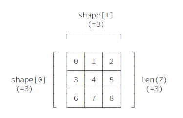
ndarray内存排布的深入理解
引子
有如下ndarray
arr = np.ones(4*1000000, np.float32)
需要将其全部赋值为8,怎么做?
%timeit arr[...] = 8
%timeit arr.view(np.float16)[...] = 8
%timeit arr.view(np.int16)[...] = 8
%timeit arr.view(np.int32)[...] = 8
%timeit arr.view(np.float32)[...] = 8
%timeit arr.view(np.int64)[...] = 8
%timeit arr.view(np.float64)[...] = 8
%timeit arr.view(np.complex128)[...] = 8
%timeit arr.view(np.int8)[...] = 8
运行时间似乎相差不大,但这种差异展示了NumPy对ndarray的内存管理的哲学。
内存排布
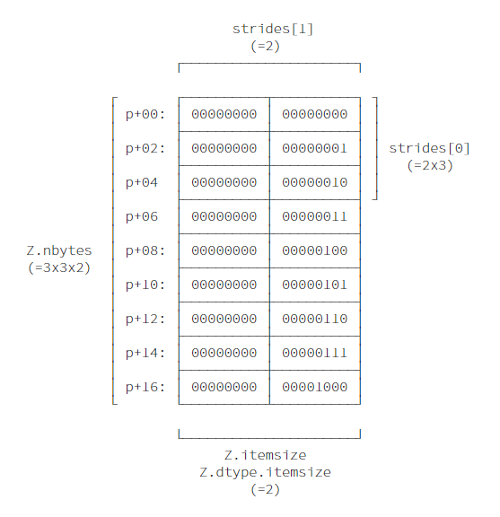
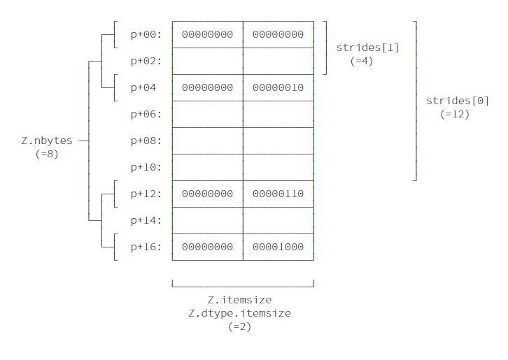
NumPy文档对ndarray的定义
An instance of class ndarray consists of a contiguous one-dimensional segment of computer memory (owned by the array, or by some other object), combined with an indexing scheme that maps N integers into the location of an item in the block.
连续的1-D内存块,搭配某种索引机制,将由整数组成的索引定位到内存块中对应的位置。
索引机制则由,形状(shape)和数据类型(data type)定义,在定义新的ndarray时也仅需这两者。
Z = np.arange(9).reshape(3, 3).astype(np.int16)
Z
Z的itemsize是2 bytes (int16), 形状为(3,3),维度为2 (len(Z.shape)).
Z.itemsize
Z.shape
Z.ndim
此外,因为Z并不是其他ndarray的视图,故可以推断出strides,即当遍历ndarray时,在每个维度上每次需要跨越多少内存。
strides = Z.shape[1]*Z.itemsize, Z.itemsize
strides
Z.strides
基于以上信息,可以确定如何索引ndarray的某个具体元素。
用tobytes方法检验一下
Z = np.arange(9).reshape(3, 3).astype(np.int16)
index = 1, 1
Z[index].tobytes()
offset_start = 0
for i in range(Z.ndim):
offset_start += Z.strides[i]*index[i]
Z.tobytes()[offset_start:offset_start + Z.itemsize]
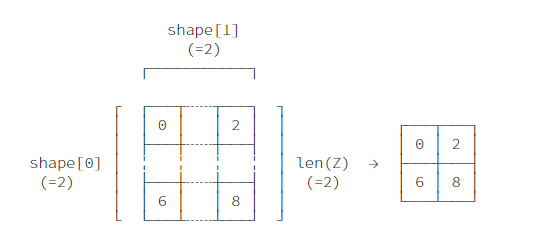
对Z进行一次切片,此时视图必须同时由形状,data type 以及 strides 才能确定,因为无法从形状和data type对strides进行推断。
V = Z[::2, ::2]
V
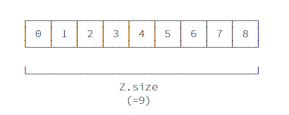
元素排布
一维化元素排布

内存排布(C order Big endian)
X = np.ones(10, dtype=np.int)
Y = np.ones(10, dtype=np.int)
A = 2*X + 2*Y # 产生三个中间变量
A
使用函数替代运算符,指定输出ndarray可以避免中间变量的产生。
X = np.ones(10, dtype=np.int)
Y = np.ones(10, dtype=np.int)
np.multiply(X, 2, out=X)
np.multiply(Y, 2, out=Y)
np.add(X, Y, out=X) # 不产生中间变量,就地操作
X
总结任务
作为总结,考虑一个任务,如果确定某个ndarray是不是另一个ndarray的视图?如果是,其start,stop,step分别是多少?
Z1 = np.arange(10)
Z2 = Z1[1:-1:2]
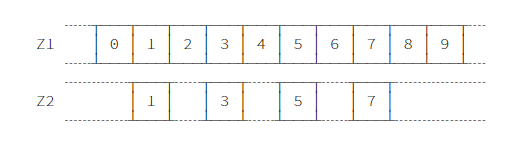
首先确定,Z2是否为Z1的视图,这个问题很好确定,只需查看Z2的base是否为Z1即可。
Z2.base is Z1
确定了Z2是Z1的视图,如何确定start,stop,step?step的确定实际上也比较简单,利用strides属性即可。
step = Z2.strides[0] // Z1.strides[0] # 注意,这里整除
step
对于start和stop,利用byte_bounds方法,该方法返回指向ndarray第一个以及最后一个元素后方的指针。
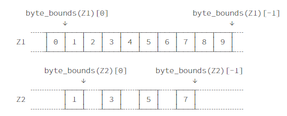
np.byte_bounds(Z1)
offset_start = np.byte_bounds(Z2)[0] - np.byte_bounds(Z1)[0]
offset_start # bytes
offset_stop = np.byte_bounds(Z2)[-1] - np.byte_bounds(Z1)[-1]
offset_stop # bytes
基于此,便可计算start,stop,step
start = offset_start // Z1.itemsize
stop = Z1.size + offset_stop // Z1.itemsize
start, stop, step
验证结果正确性
np.allclose(Z1[start:stop:step], Z2)
进阶任务
以上任务仅针对一维ndarray而言,且未考虑负数step的情况,考虑多维ndarray以及负数step则
Z1 = np.ones((5, 5))
Z2 = Z1[::2, ::2]
Z2
itemsize = Z2.itemsize
offset_start = (np.byte_bounds(Z2)[0] - np.byte_bounds(Z1)[0])//itemsize
offset_stop = (np.byte_bounds(Z2)[-1] - np.byte_bounds(Z1)[-1]-1)//itemsize
index_start = np.unravel_index(offset_start, Z1.shape)
index_stop = np.unravel_index(Z1.size+offset_stop, Z1.shape)
index_step = np.array(Z2.strides)//np.array(Z1.strides)
index_start, index_stop, index_step
index = np.empty((Z1.ndim, 3)).astype(np.int16)
for i in range(len(index_step)):
start = index_start[i]
stop = index_stop[i]
step = index_step[i]
if step < 0:
start, stop = stop, start - 1
else:
start, stop = start, stop + 1
index[i] = start, stop, step
index